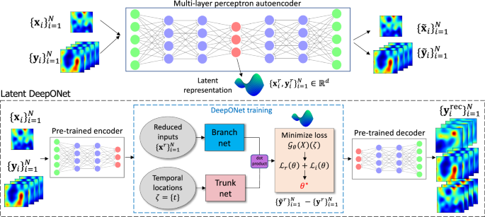
To demonstrate the advantages and efficiency of L-DeepONet, we learn the operator for three diverse PDE models of increasing complexity and dimensionality. First, we consider a PDE that describes the growth of fracture in brittle materials which are widely used in various industries including construction and manufacturing. Predicting with accuracy the growth of fractures in these materials is important for preventing failures, improving safety, reliability, and cost-effectiveness in a wide range of applications. Second, we consider a PDE describing convective fluid flow, a common phenomenon in many natural and industrial processes. Understanding how these flows evolve may allow engineers to better design systems such as heat exchangers or cooling systems to enhance efficiency and reduce energy consumption. Finally, we consider a PDE describing large-scale atmospheric flows which can be used to predict patterns that occur in weather systems. Such flows play a crucial role in the Earth’s climate system influencing precipitation, and temperature which in turn may have a significant impact on water resources, agricultural productivity, and energy production. Developing an accurate surrogate to predict with detail such complex atmospheric patterns may allow us to better adapt to changes in the climate system and develop effective strategies to mitigate the impacts of climate change. For all PDEs, the input functions for the operator represent initial conditions modeled as Gaussian or non-Gaussian random fields. We perform direct comparisons of L-DeepONet with the standard DeepONet model trained on the full dimensional data and with FNO. More details about the models and the corresponding data generation process are provided in the Supplementary Section on Data Generation to assist the readers in readily reproducing the results presented below.
Brittle fracture in a plate loaded in shear
Fracture is one of the most commonly encountered failure modes in engineering materials and structures. Defects, once initialized, can lead to catastrophic failure without warning. Therefore, from a safety point of view, prediction of the initiation and propagation of cracks is of utmost importance. In the phase field fracture modeling approach, the effects associated with crack formation, such as stress release, are incorporated into the constitutive model43. Modeling fracture using the phase field method involves the integration of two fields, namely the vector-valued elastic field, u(x), and the scalar-valued phase field, \(\phi \left({{{{{{{\boldsymbol{x}}}}}}}}\right)\in [0,1]\), with 0 representing the undamaged state of the material and 1 a fully damaged state.
The equilibrium equation for the elastic field for an isotropic model, considering the evolution of crack, can be written as44:
$$-\nabla \cdot g(\phi ){{{{{{{\boldsymbol{\sigma }}}}}}}}={{{{{{{\boldsymbol{f}}}}}}}}\,{{{{{{{\rm{on}}}}}}}}\,\Omega,$$
(1)
where σ is the Cauchy stress tensor, f is the body force and g(ϕ) = (1−ϕ)2 represents the monotonically decreasing stress-degradation function that reduces the stiffness of the bulk material in the fracture zone. The elastic field is constrained by Dirichlet and Neumann boundary conditions:
$$g(\phi ){{{{{{{\boldsymbol{\sigma }}}}}}}}\cdot {{{{{{{\boldsymbol{n}}}}}}}} ={{{{{{{{\boldsymbol{t}}}}}}}}}_{N}\,{{{{{{{\rm{on}}}}}}}}\,\partial {\Omega }_{N},\\ {{{{{{{\boldsymbol{u}}}}}}}} ={{{\overline{{{{{\boldsymbol{u}}}}}}}}}\,{{{{{{{\rm{on}}}}}}}}\,\partial {\Omega }_{D},$$
(2)
where tN is the prescribed boundary forces and \({{{\overline{{{{{\boldsymbol{u}}}}}}}}}\) is the prescribed displacement for each load step. The Dirichlet and Neumann boundaries are represented by ∂ΩD and ∂ΩN, respectively. Considering the second-order phase field for a quasi-static setup, the governing equation can be written as:
$$\frac{{G}_{c}}{{l}_{0}}\phi -{G}_{c}{l}_{0}{\nabla }^{2}\phi=-{g}^{{\prime} }(\phi )H({{{{{{{\boldsymbol{x}}}}}}}},t;{l}_{c},{y}_{c})\,{{{{{{{\rm{on}}}}}}}}\,\Omega,$$
(3)
where Gc is a scalar parameter representing the critical energy release rate of the material, l0 is the length scale parameter, which controls the diffusion of the crack, H(x, t) is a local strain-history functional, and yc, lc represent the position and length of the crack respectively. For sharp crack topology, l0 → 045. H(x, t) contains the maximum positive tensile energy (\({\Psi }_{0}^{+}\)) in the history of deformation of the system. The strain-history functional is employed to initialize the crack on the domain as well as to impose irreversibility conditions on the crack growth46. In this problem, we consider yc, lc to be random variables with yc ~ U[0.3, 0.7] and lc ~ U[0.4, 0.6], thus, the initial strain function H(x, t = 0; lc, yc) is also random (see the Supplementary Section on Data Generation). We aim to learn the solution operator \({{{{{{{\mathscr{G}}}}}}}}:H({{{{{{{\boldsymbol{x}}}}}}}},t=0;{l}_{c},{y}_{c})\mapsto \phi ({{{{{{{\boldsymbol{x}}}}}}}},t)\) which maps the initial strain-history function to the crack evolution.
In Fig. 2a, we show the mean-square error (MSE) between the studied models and ground truth. The left panel shows the MSE for the multi-layer autoencoder (MLAE) for different latent dimensions (d), where the violin plot shows the distribution of MSE from n = 5 independent trials. The right panel shows the resulting MSE for L-DeepONet operating on different latent dimensions (d) compared with the full high-dimensional DeepONet, FNO-2D, and FNO-3D. We observe that, regardless of the latent dimension, the L-DeepONet outperforms the standard DeepONet (Full DON) and performs comparably with FNO-2D and FNO-3D. In Fig. 3, a comparison between all models for a random representative result is shown. While L-DeepONet results in prediction fields almost identical to the reference, the predictions of the standard models deviate from the ground truth both inside and around the propagated crack. Finally, the cost of training the different models is presented in Table 1. Because the required network complexity is significantly reduced, the L-DeepONet is 1 − 2 orders of magnitude cheaper to train than the standard approaches.
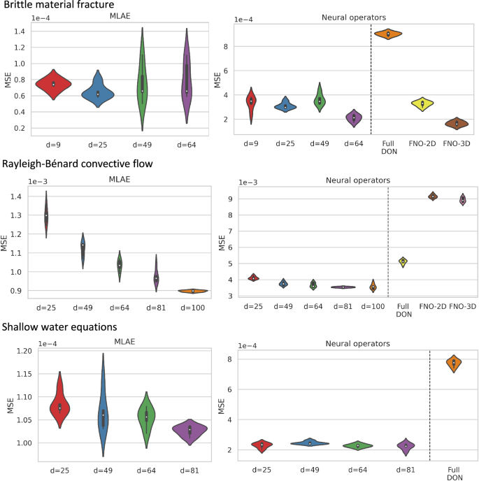
Left: Results for the multi-layer autoencoders (MLAE) for different values of the latent dimensionality. Right: Results for all the studied neural operators. For all panes, violin plots are generated from 5 independent trainings of the models using different random seed numbers.
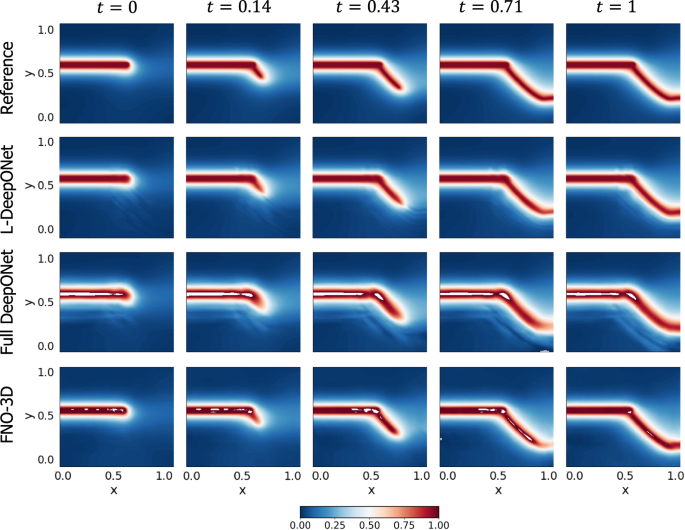
The results of the L-DeepONet model consider the latent dimension, d = 64. The neural operator is trained to approximate the growth of the crack for five time steps from a given initial location of the defect.
Rayleigh-Bénard fluid flow convection
Rayleigh-Bénard convection occurs in a thin layer of fluid that is heated from below47. The natural fluid convection is buoyancy-driven and caused due to a temperature gradient ΔT. Instability in the fluid occurs when ΔT is large enough to make the non-dimensional Rayleigh number, Ra, exceed a certain threshold. The Rayleigh number whose physical interpretation is the ratio between the buoyancy and the viscous forces is defined as
$${{{{{{{\rm{Ra}}}}}}}}=\frac{\alpha \Delta Tg{h}^{3}}{\nu \kappa },$$
(4)
where α is the thermal expansion coefficient, g is the gravitational acceleration, h is the thickness of the fluid layer, ν is the kinematic viscosity and κ is the thermal diffusivity. When ΔT is small, the convective flow does not occur due to the stabilizing effects of viscous friction. Based on the governing conservation laws for an incompressible fluid (mass, momentum, energy) and the Boussinesq approximation according to which density perturbations affect only the gravitational force, the dimensional form of the Rayleigh-Bénard equations for a fluid defined on a domain Ω reads:
$$\left\{\begin{array}{ll}\frac{{{{{{{{\rm{D}}}}}}}}{{{{{{{\boldsymbol{u}}}}}}}}}{{{{{{{{\rm{D}}}}}}}}t}=-\frac{1}{{\rho }_{0}}\nabla p+\frac{\rho }{{\rho }_{0}}g+\nu {\nabla }^{2}{{{{{{{\boldsymbol{u}}}}}}}},\quad &{{{{{{{\boldsymbol{x}}}}}}}}\in \Omega,t \, > \,0,\\ \frac{{{{{{{{\rm{D}}}}}}}}T}{{{{{{{{\rm{D}}}}}}}}t}=\kappa {\nabla }^{2}T,\hfill\quad&{{{{{{{\boldsymbol{x}}}}}}}}\in \Omega,t \, > \,0,\\ \nabla \cdot {{{{{{{\boldsymbol{u}}}}}}}}=0,\hfill\quad &\\ \rho={\rho }_{0}(1-\alpha (T-{T}_{0})),\hfill\quad &\end{array}\right.$$
(5)
where D/Dt denotes material derivative, u, p, T are the fluid velocity, pressure and temperature respectively, T0 is the temperature at the lower plate, and x = (x, y) are the spatial coordinates. Considering two plates (upper and lower) the corresponding BCs and ICs are defined as
$$\left\{\begin{array}{ll}T({{{{{{{\boldsymbol{x}}}}}}}},t){| }_{y=0}={T}_{0},\hfill\quad &{{{{{{{\boldsymbol{x}}}}}}}}\in \Omega,t \, > \,0,\\ T({{{{{{{\boldsymbol{x}}}}}}}},t){| }_{y=h}={T}_{1},\hfill\quad &{{{{{{{\boldsymbol{x}}}}}}}}\in \Omega,t \, > \,0,\\ {{{{{{{\boldsymbol{u}}}}}}}}({{{{{{{\boldsymbol{x}}}}}}}},t){| }_{y=0}={{{{{{{\boldsymbol{u}}}}}}}}({{{{{{{\boldsymbol{x}}}}}}}},t){| }_{y=h}=0,\hfill\quad &{{{{{{{\boldsymbol{x}}}}}}}}\in \Omega,t \, > \,0,\\ T(y,t){| }_{t=0}={T}_{0}+\frac{y}{h}({T}_{1}-{T}_{0})+0.1v({{{{{{{\boldsymbol{x}}}}}}}}),\quad &{{{{{{{\boldsymbol{x}}}}}}}}\in \Omega,\\ {{{{{{{\boldsymbol{u}}}}}}}}({{{{{{{\boldsymbol{x}}}}}}}},t){| }_{t=0}=0,\quad &{{{{{{{\boldsymbol{x}}}}}}}}\in \Omega,\end{array}\right.$$
(6)
where T0, and T1 are the fixed temperatures of the lower and upper plates, respectively. For a 2D rectangular domain and through a non-dimensionalization of the above equations, the fixed temperatures become T0 = 0 and T1 = 1. The IC of the temperature field is modeled as linearly distributed with the addition of a GRF, v(x) having correlation length scales ℓx = 0.45, ℓy = 0.4 simulated using a Karhunen-Loéve expansion. The objective is to approximate the operator \({{{{{{{\mathscr{G}}}}}}}}:T({{{{{{{\boldsymbol{x}}}}}}}},t=0)\mapsto T({{{{{{{\boldsymbol{x}}}}}}}},t)\) (see the Supplementary Section on Data Generation).
Figure 2b again shows violin plots of the MSE for the MLAE with differing latent dimensions and the MLE for the corresponding L-DeepONet compared with the other neural operators. Here we see that the reconstruction accuracy of the MLAE is improved by increasing the latent dimensionality up to d = 100. However, the change in the predictive accuracy of L-DeepONet for different values of d is less significant, indicating that latent spaces with even very small dimensions (d = 25) result in a very good performance. Furthermore, L-DeepONet outperforms all other neural operators with a particularly significant improvement compared to FNO. In Fig. 4, we observe that L-DeepONet is able to capture the complex dynamical features of the true model with high accuracy as the simulation evolves. In contrast, the standard DeepONet and FNO result in diminished performance as they tend to smooth out the complex features of the true temperature fields. Furthermore, the training time of the L-DeepONet is significantly lower than the full DeepONet and FNO as shown in Table 1.
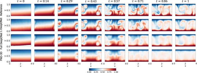
The results of the L-DeepONet model consider the latent dimension, d = 100. The neural operator is trained to approximate the growth of the evolution of the temperature field from a realization of the initial temperature field for seven time steps.
Shallow-water equations
The shallow-water equations model the dynamics of large-scale atmospheric flows48. In a vector form, the viscous shallow-water equations can be expressed as
$$\left\{\begin{array}{l}\frac{{{{{{{{\rm{D}}}}}}}}{{{{{{{\boldsymbol{V}}}}}}}}}{{{{{{{{\rm{D}}}}}}}}t}=-f{{{{{{{\boldsymbol{k}}}}}}}}\times {{{{{{{\boldsymbol{V}}}}}}}}-g\nabla h+\nu {\nabla }^{2}{{{{{{{\boldsymbol{V}}}}}}}},\hfill\quad \\ \frac{{{{{{{{\rm{D}}}}}}}}h}{{{{{{{{\rm{D}}}}}}}}t}=-h\nabla \cdot {{{{{{{\boldsymbol{V}}}}}}}}+\nu {\nabla }^{2}h,\quad {{{{{{{\boldsymbol{x}}}}}}}}\in \Omega,t\in [0,1],\quad \end{array}\right.$$
(7)
where Ω = (λ, ϕ) represents a spherical domain where λ, ϕ are the longitude and latitude respectively ranging from [ − π, π], V = iu + jv is the velocity vector tangent to the spherical surface (i and j are the unit vectors in the eastward and northward directions respectively and u, v the velocity components), and h is the height field which represents the thickness of the fluid layer. Moreover, \(f=2\Xi \sin \phi\) is the Coriolis parameter, where Ξ is the Earth’s angular velocity, g is the gravitational acceleration and ν is the diffusion coefficient.
As an initial condition, we consider a zonal flow which represents a typical mid-latitude tropospheric jet. The initial velocity component u is expressed as a function of the latitude ϕ as
$$u(\phi,t=0)=\left\{\begin{array}{ccl}0&{{{{{{{\rm{for}}}}}}}}&\phi \,\le \,{\phi }_{0},\\ \frac{{u}_{\max }}{n}\,\exp \left[\frac{1}{(\phi -{\phi }_{0})(\phi -{\phi }_{1})}\right]&{{{{{{{\rm{for}}}}}}}}&{\phi }_{0} \, < \,\phi \, < \,{\phi }_{1},\\ 0&{{{{{{{\rm{for}}}}}}}}&\phi \,\ge \,{\phi }_{1},\end{array}\right.$$
(8)
where \({u}_{\max }\) is the maximum zonal velocity, ϕ0, and ϕ1 represent the latitude in the southern and northern boundary of the jet in radians, respectively, and \(n=\exp [-4/{({\phi }_{1}-{\phi }_{0})}^{2}]\) is a non-dimensional parameter that sets the value \({u}_{\max }\) at the jet’s mid-point. A small unbalanced perturbation is added to the height field to induce the development of barotropic instability. The localized Gaussian perturbation is described as
$${h}^{{\prime} }(\lambda,\phi,t=0)=\hat{h}\cos (\phi )\exp [-{(\lambda /\alpha )}^{2}]\exp {[-({\phi }_{2}-\phi )/\beta ]}^{2},$$
(9)
where − π < λ < π and \(\hat{h},{\phi }_{2},\alpha,\beta\) are parameters that control the location and shape of the perturbation. We consider α, β to be random variables with \(\alpha \sim U[0.\bar{1},0.5]\) and \(\beta \sim U[0.0\bar{3},0.2]\) so that the input Gaussian perturbation is random. The localized perturbation is added to the initial height field, which forms the final initial condition h(λ, ϕ, t = 0) (see Supplementary Section on Data Generation). The objective is to approximate the operator \({{{{{{{\mathscr{G}}}}}}}}:h(\lambda,\phi,t=0)\mapsto u(\lambda,\phi,t)\). This problem is particularly challenging as the fine mesh required to capture the details of the convective flow both spatially and temporally results in output realizations having millions of dimensions.
Unlike the previous two applications, here the approximated operator learns to map the initial condition of one quantity, h(λ, ϕ, t = 0), to the evolution of a different quantity, u(λ, ϕ, t). Given the difference between the input and output quantities of interest (in scale and features), a single encoding of the combined data as in the standard proposed approach (see Fig. 1) is insufficient. Instead, two separate encodings are needed for the input and output data, respectively. While an autoencoder is used to reduce the dimensionality of the output data representing the longitudinal component of the velocity vector u, standard principal component analysis (PCA) is performed on the input data due to the small local variations in the initial random height field h which results in a small intrinsic dimensionality.
Results, in terms of MSE, are presented in Fig. 2c, where again we see that the L-DeepONet outperforms the standard approach while changes in the latent dimension do not result in significant differences in the model accuracy. Consistent with the results of the previous application, the training cost of the L-DeepONet is much lower than the full DeepONet (Table 1). We further note that training FNO for this problem (either FNO-2D or FNO-3D) proved computationally prohibitive. For a moderate 3D problem with spatial discretization beyond 643, the latest GPU architectures such as the NVIDIA Ampere GPU do not provide sufficient memory to process a single training sample49. Data partitioning across multiple GPUs with distributed memory, model partitioning techniques like pipeline parallelism, and domain decomposition approaches49 can be implemented to handle high-dimensional tensors within the context of an automatic differentiation framework to compute the gradients/sensitivities of PDEs and thus optimize the network parameters. This advanced implementation is beyond the scope of this work as it proves unnecessary for the studied approach. Consequently, a comparison to the FNO is not shown here. A variant of FNO, the Spherical Fourier neural operator (S-FNO) has been tailored for problems on spherical domains such as shallow water equations50. However, S-FNO is primarily focused on mapping the initial condition to the solution at a final timestamp. In contrast, our objective is to learn the mapping from the initial condition to the solution time history, enabling the generation of a sequence of solutions at arbitrary time instants. Hence, we have not provided a comparison between L-DeepONet and S-FNO for this problem. Figure 5, shows the evolution of the L-DeepONet and the full DeepONet compared to the ground truth for a single realization. The L-DeepONet consistently captures the complex nonlinear dynamical features for all time steps, while the full model prediction degrades over time and again smoothing the results such that it fails to predict extreme velocity values for each time step that can be crucial, e.g., in weather forecasting.
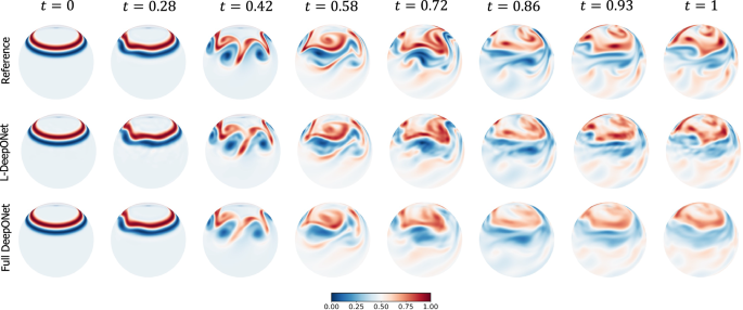
The results of the L-DeepONet model consider the latent dimension, d = 81.


